You Can Now Use SQL in Excel! (This Changes Everything)

Introduction
You can now use SQL formulas directly in Microsoft Excel. Just like in my example here, I’ve added an SQL formula to group my orders table by customer ID and then calculate the total amount spent by each customer. This, of course, is just one example. With SQL, you can do almost anything when it comes to extracting and transforming structured data. In the past, I made a similar video, but back then we needed Python installed on our computer to make it work. Now, with this new solution, all you need is a free Excel add-in called SQLOOKUP. It works right out of the box on Windows, Mac, and even the web version of Excel. In this post, I will show you how to get started with the add-in and how to use it.
Installing the SQLOOKUP Add-In
First things first, we need to install the add-in. To do that, go to the home tab and navigate to add-ins. From here, search for SQLOOKUP. Once you find it, click on add. That’s it! We have now installed the add-in. If you look under the Formulas tab, you will now see the SQLOOKUP icon. Clicking on it will open the task pane. 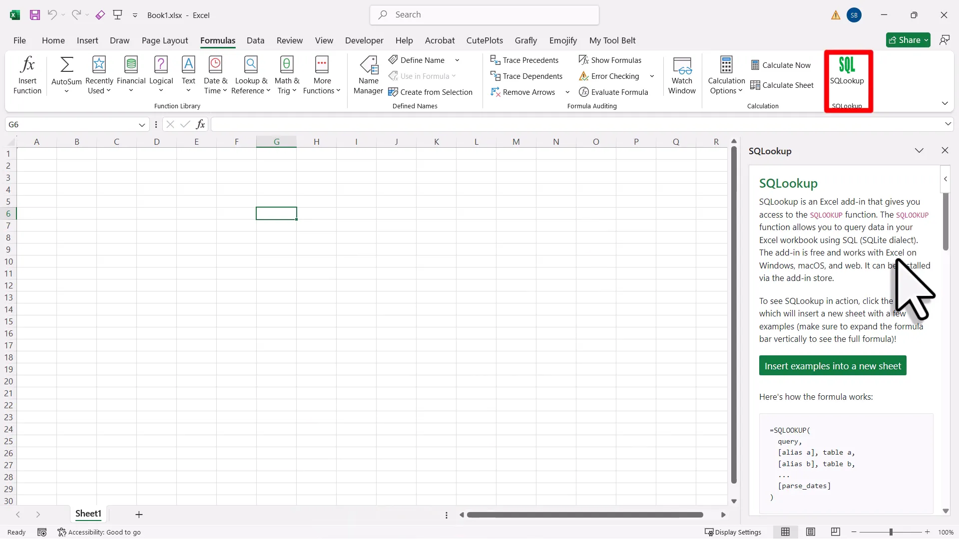
Using SQLOOKUP to Query Data
Now let me insert some sample data into our sheet so that we can see how it works. Here we have two tables: one contains customer data and the other contains some sample order data. With the add-in installed, we now have a new formula called SQLOOKUP, which lets you write SQL queries directly in Excel. For a simple example, let’s say I want to get all the customers from New York. To do that, I will write an SQL statement inside the SQLOOKUP formula. I will select everything from the table and add a filter criterion for the city. For the table name, you can simply use the letter A. After that, select the range of your table. This can be either an actual Excel table or a range of cells. 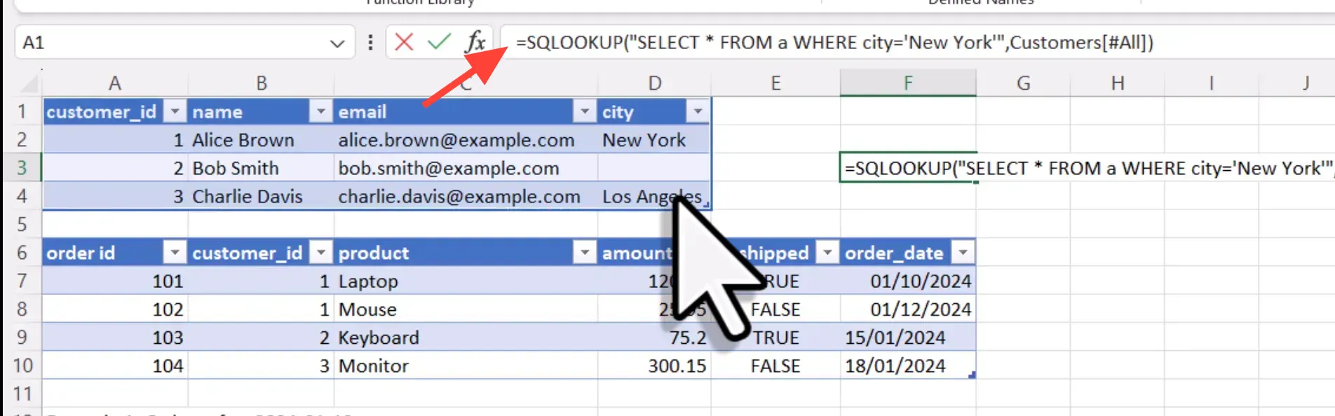
Improving Readability
To make things more readable, I will give this table a proper name. Instead of using the letter A, I will call it CustomersTable. When you do this, you also need to specify the table name in the formula. In quotation marks, I will type CustomersTable, and the range for this will be my table called Customers. When I press enter, we can see that it still works. To improve the readability even further, you can also write your SQL statements in multiple lines. In Excel, you can do this by pressing Alt and Enter to insert a line break inside the formula. You don’t actually need to capitalize the SQL keywords, although I do it here to make the statement easier to read. 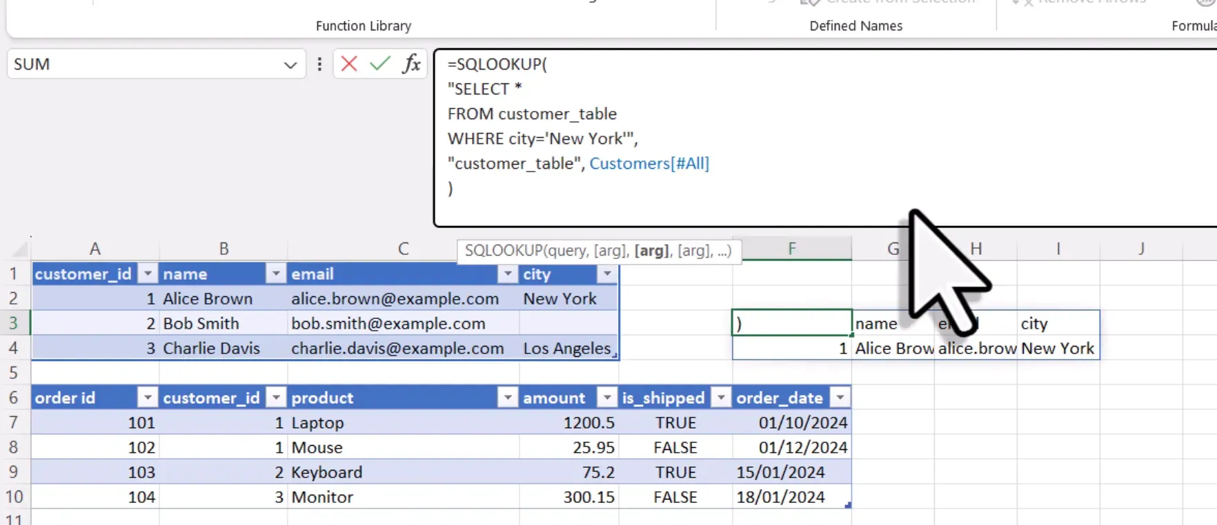
Making Formulas Dynamic
Next, let’s make this formula a bit more dynamic. Instead of hardcoding the filter criterion for the city directly into the SQL formula, I want to reference it from a separate cell. I will create a small input field where I can type in the city name, using cell G2 for this. In the SQL formula, we will use string concatenation to include the input field as part of the query. Right now, the SQL statement is just one long string. To insert the variable, I will break the string by adding quotation marks and using the ampersand to concatenate it with the rest of the formula. With that in place, I can replace the hard-coded New York with the reference cell in G2. When I press enter, we can see that it still works. 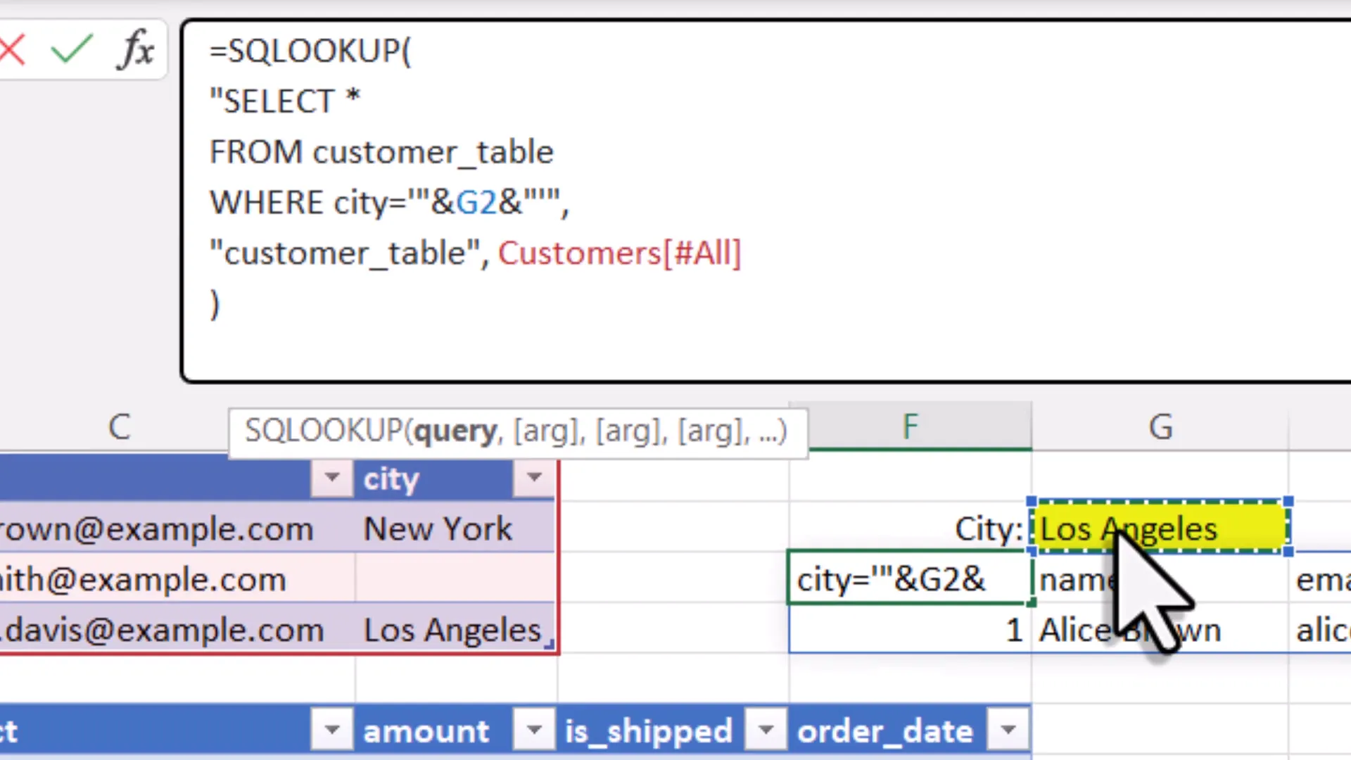
Filtering Orders by Date
Currently, I am still seeing a spill error, which just means there is not enough space for our result. I will insert a new row here to give the results room to display. In this example, we are filtering the orders table by the order date column. The table name orders is defined here and it references the order table in our sheet. To test it out, let’s filter the data to only show the orders after the 1st of July. When I press enter, we can see the result, and only two orders match our criteria. 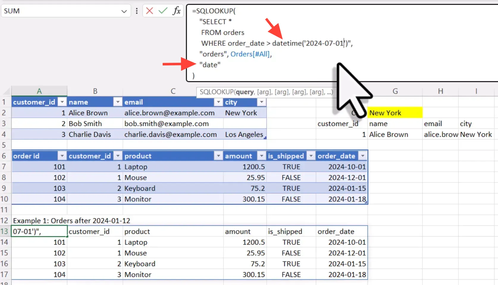
Understanding SQL Dialect
One important note here: this add-in uses the SQLite dialect under the hood. That is why you have access to the functions’ date and time in your SQL statements. If you want to see all the available SQLite functions, you can check out their documentation. For example, under the date and time section, you will find the date time function we just used. 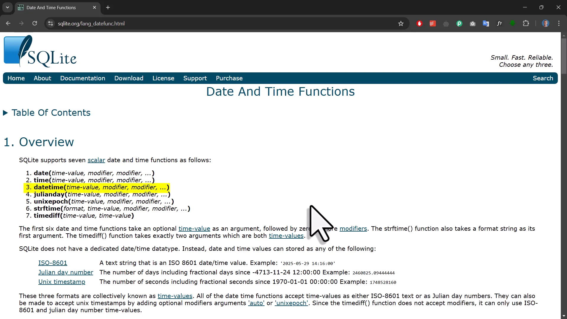
Working with Joins
Here we are working with two tables and performing an inner join. The order table has an alias of O and the customer table is alias as C. In the SQL statement, we can reference those tables. This allows us to perform more complex queries that involve multiple tables. 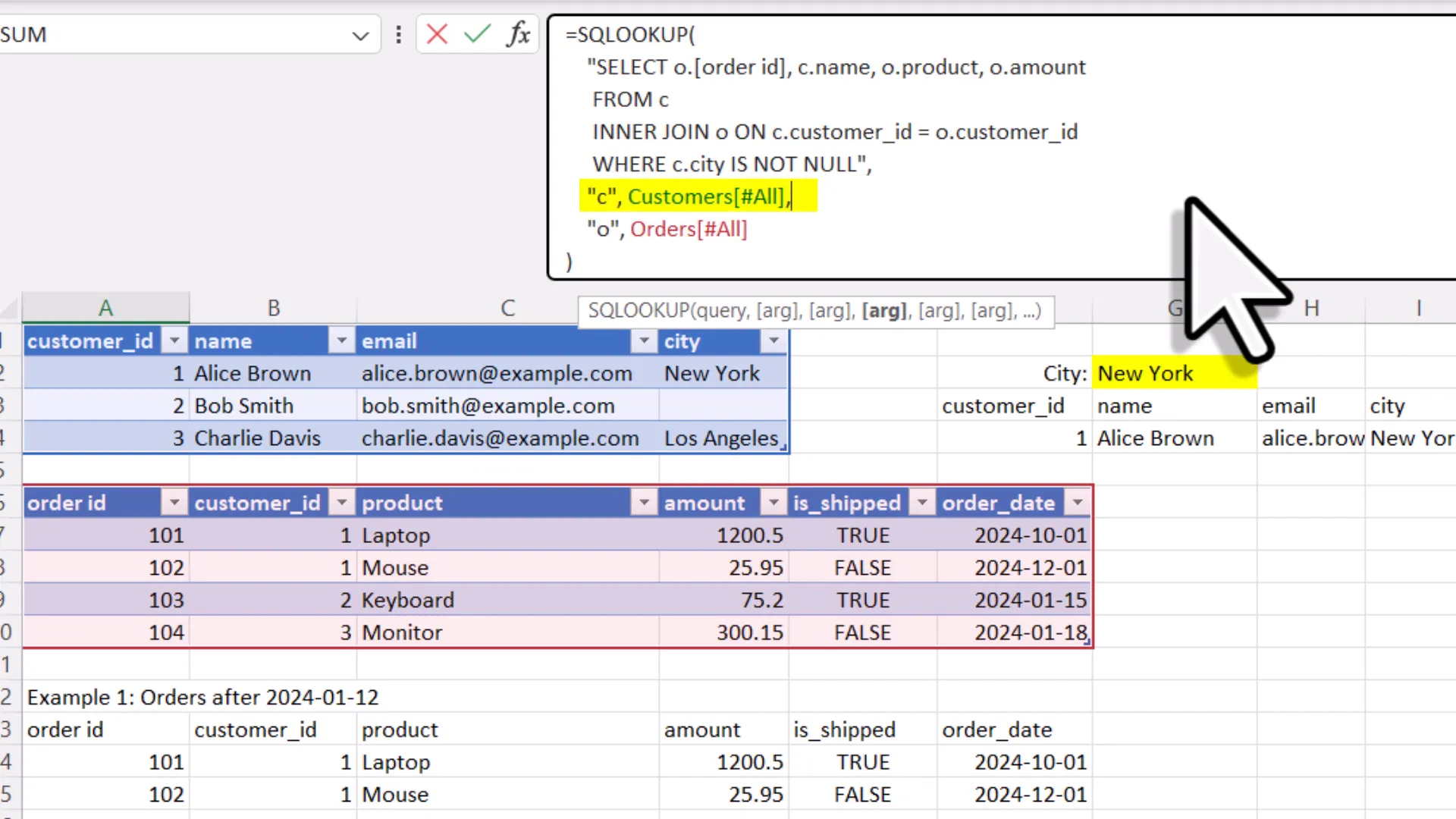
Using Group By to Summarize Data
In the final example, we are using a group by statement to summarize the data. We are grouping it by the customers and calculating the total spending in a new column called total spend. This allows for easy data summarization directly within Excel. 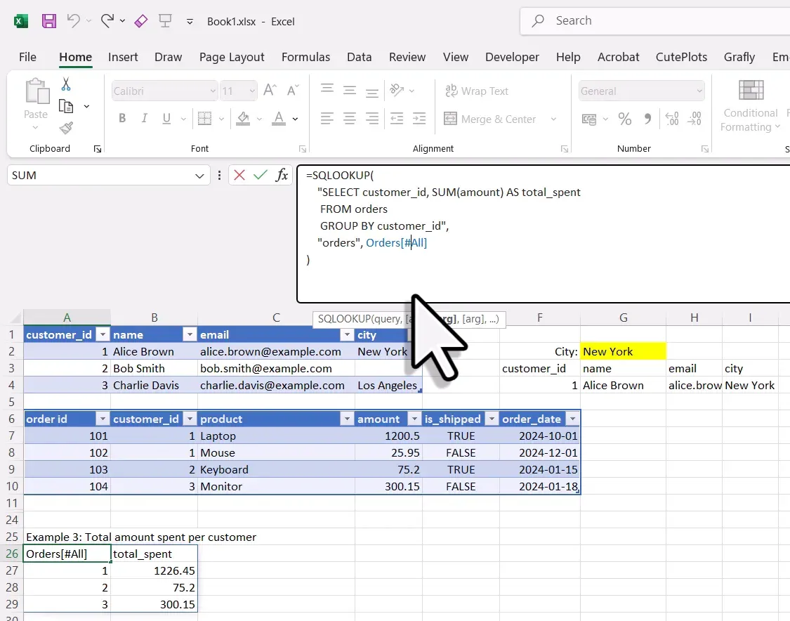
Handling Add-In Deletion
You might be wondering what happens if you delete the add-in or send this workbook to someone who doesn’t have the add-in installed. After removing the add-in, the results are still visible in my workbook. However, if I try to recalculate the formula, it shows a name error, meaning that the formula can no longer run. 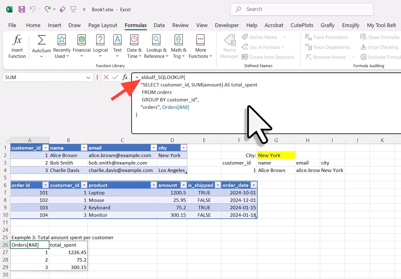
Privacy and Security
Lastly, let’s talk about privacy. The SQL queries actually run locally on your machine, meaning no data is sent to an external server. Additionally, the add-in doesn’t collect any user statistics, so it is pretty safe to use. 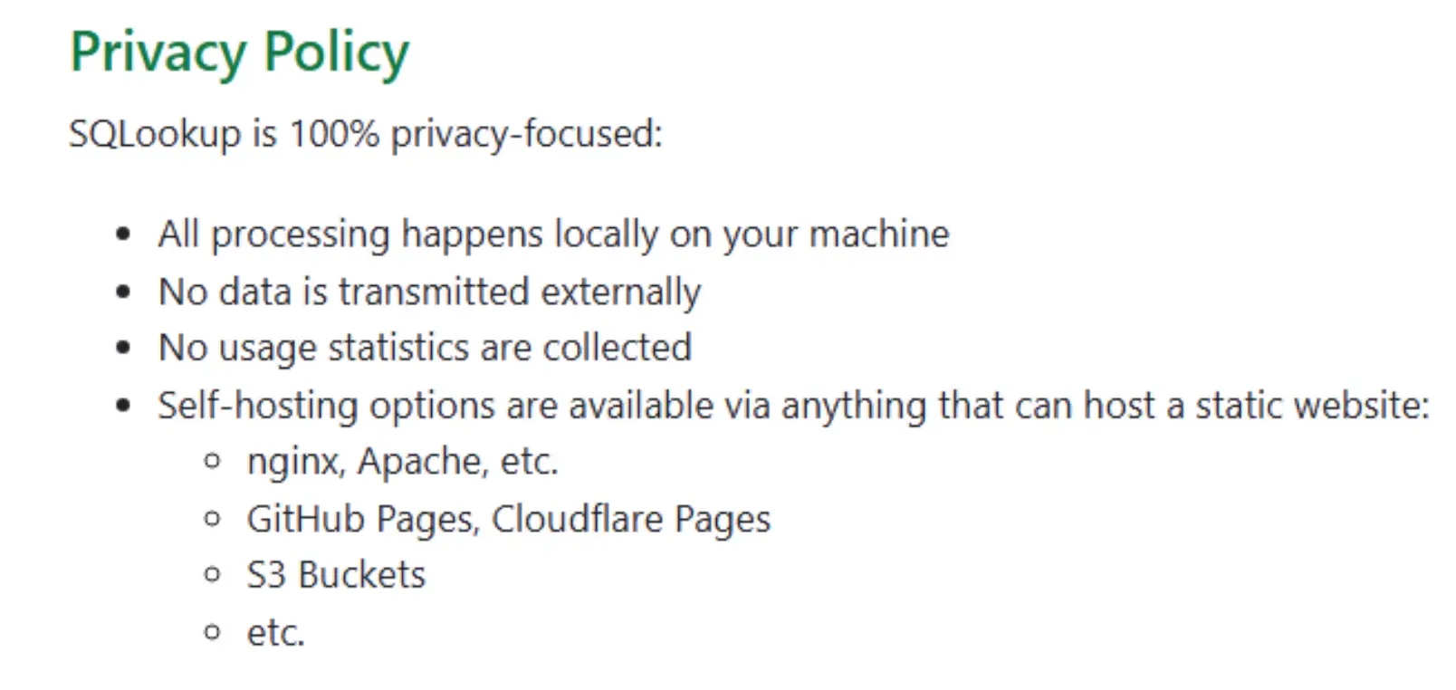
Conclusion
In this post, I covered how to use the SQLOOKUP add-in to run SQL queries directly in Excel, from installation to practical examples of filtering, joining, and summarizing data. This tool opens up new possibilities for data analysis within Excel, making it more powerful and efficient. Thanks for reading.