
Matching takes two lists that describe the same things in different ways, for example customers in your CRM and vendors in your accounting system, and finds for every row of the first list the same business, organization or person in the second list.
- List A holds the records you want to match. Every row gets a result.
- List B is the reference list the matches come from.
1. Pick List A #
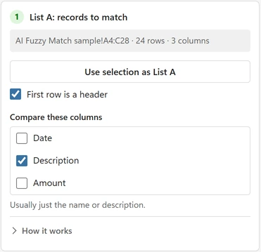
Click any cell inside your first list and click Use selection as List A. One cell is enough: the add-in takes the whole block of data around it and shows the address, the number of rows and the number of columns. The first row is read as headers; if your list has no headers, the pane asks you to confirm before it continues.
Then tick the columns under Compare these columns, usually just the name. See Choose the columns to compare.
2. Pick List B #
Do the same for the reference list with Use selection as List B. Here you choose two things: The AI picks from these columns (again, usually just the name), and Copy these columns next to List A, for example a vendor ID.
3. Check the estimate and run #
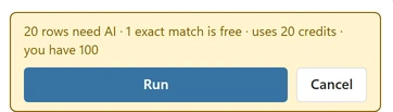
Optionally, write an extra rule first (see below). Click Check credits and run: the pane shows how many rows need the AI, how many are exact matches (free) and how many credits that uses. Nothing runs until you confirm. The confidence threshold (default 80%) and where the results go are in Settings; see Where the results go.
While it runs, the pane shows the progress and writes results as they arrive. Cancel stops cleanly and keeps every row that is already done.
Extra rule (optional) #
Step 3 has an Extra rule field for one instruction of up to 200 characters. The AI adds it to its usual question for every row. Leave it empty for normal matching. Examples:
- “Branches of the same company count as one”
- “A subsidiary is not the same as its parent company”
- “Size, colour and pack size must match”
- “The seniority level must match”
The AI applies the rule to every column you compare, so name the column: write “The house number must match”, not “Numbers must match”. Click an example under the field to use it.
Use “A subsidiary is not the same as its parent company” for a vendor master clean-up, where a subsidiary that is missing from List B (Microsoft Canada Inc., say) would otherwise be matched to its parent’s vendor number. The rule costs nothing extra. The AI gets stricter with it, so a few borderline rows, such as abbreviations and renamed companies, may go to Review.
The rule is saved with the workbook. It is sent with the rows, and the matching service does not log or store it. If you change the rule and some rows already have a result made with the old one, the pane asks whether to redo those rows or keep them.
4. Read the results #
The add-in adds these columns, by default next to List A:
- Match: the entry from List B, or empty when there is no match.
- Confidence: how sure the AI is, as a percentage from 0% to 100%.
- Status: one of the values below.
- <column> (matched): one column for each List B column you chose to copy, for example “Vendor ID (matched)”.
| Status | What it means |
|---|---|
| Matched | The AI chose an entry with a confidence at or above your threshold. |
| Review | The AI answered below your threshold, with an entry or with No match. By default these rows get a light yellow fill. Check them. |
| No match | None of the entries in List B is the same business, organization or person. See Why did a row get No match? |
| Exact | The row is identical to exactly one entry in List B after a cleanup of case, accents, punctuation and legal suffixes. Matched inside Excel, free. |
| Duplicate in List B | The same entry text appears more than once in List B, so the add-in cannot tell which of those rows you mean. The copied “(matched)” columns stay empty on this row, unless all of those List B rows hold the same value, so no possibly wrong ID lands in your sheet. Pick the right row yourself, or tick another column such as City so each entry is unique. |
At the end, the pane sums it up in one line, for example: “3,200 rows · 2,410 matched · 280 to review · 510 no match”. Show review rows filters your list to the rows that need a look.
Where the results go #
Open the menu (top left) and go to Settings. Under Results, Results go has three options:
- Next to List A (the default): new empty columns right of List A. If List A is an Excel table, Excel may widen the table to take them in.
- Starting at column: on List A’s sheet, in List A’s header row, from the Column letter you enter.
- On a new sheet: a sheet named “AI Fuzzy Match results” with a copy of the List A columns you compare. List A’s sheet is not changed.
Highlight rows to review is on by default: Review and Duplicate in List B rows get a light yellow fill in the result columns. Turn it off for no fill; the Status column and Show review rows still work.
Results never overwrite cells that hold data. Changes apply to the next run.
Running again and clearing #
- A second run skips rows that already have a result, so an interrupted run simply continues. When every row already has a result, the pane offers Redo all rows to answer every row again (this uses credits again).
- Clear results removes only the result columns the add-in wrote, after asking you. Your own data is never changed.
Limits #
Up to 50,000 rows in List A per run and up to 100,000 rows in List B. For lists in the thousands, read Work with big lists.